Real-time dashboard¶

File: demo/realtime_dashboard.m.

A uifigure-based dashboard that runs the 50 mg baseline and 60 mg modified dose back-to-back with Simulink Pacing enabled so the model plays out in near real time, then overlays the two runs in a single comparison view.

This is Prompt 8 in the demo sequence: the visualisation closer that turns the numerical comparison from Prompt 4 into something a non-engineer can absorb at a glance.

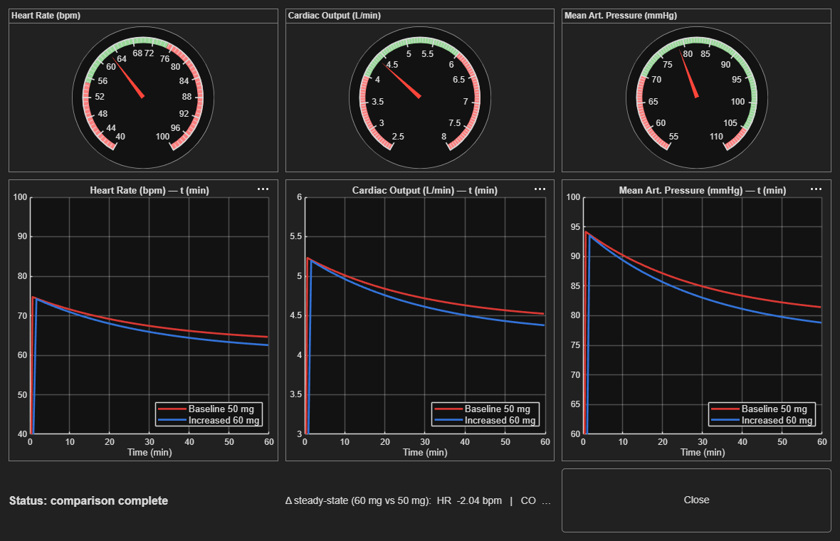
Real-time dashboard showing both 50 mg and 60 mg runs overlaid

Final dashboard state after both runs complete. Gauges show the live 60 mg values (HR 66.6, CO 4.66, MAP 83.9). The time-history axes overlay the two runs: red is 50 mg baseline, blue is 60 mg modified. The delta strip at the bottom shows the steady-state difference.

Layout¶

+----------------------------------------------------+
|   [HR gauge]    [CO gauge]    [MAP gauge]          |   <-- live current values
|                                                    |
|   [HR axes]     [CO axes]     [MAP axes]           |   <-- both runs overlaid
|                                                    |
|   Status: ...                                      |
|   Δ steady-state (60 vs 50): HR ... CO ... MAP ... |
|   [Close]                                          |
+----------------------------------------------------+

Component	Role
Three `uigauge` widgets	Current HR, CO, MAP. Re-coloured per run so you see the now-value.
Three `uiaxes` with `animatedline`	Time history. Run 1 drawn in red, run 2 drawn in blue, both retained for comparison.
Status label	Tells the viewer which run is currently executing.
Δ readout	After both runs complete, shows the steady-state delta on all three outputs.

How the live update works¶

The dashboard does not simulate in batch and replay. It uses the live simulation engine and polls the running model:

set_param(mdl, 'EnablePacing', 'on', 'PacingRate', '200', 'StopTime', '3600');
set_param(mdl, 'ReturnWorkspaceOutputs', 'off');

HR_block  = [mdl '/HeartRateModel/HRClamp'];      % leaf Saturation block
CO_block  = [mdl '/CardiacOutputModel/mLtoL'];    % leaf Gain block
MAP_block = [mdl '/BloodPressureModel/SVRGain'];  % leaf Gain block

set_param(mdl, 'SimulationCommand', 'start');

while ~strcmp(get_param(mdl, 'SimulationStatus'), 'stopped')
    rto_hr  = get_param(HR_block,  'RuntimeObject');
    rto_co  = get_param(CO_block,  'RuntimeObject');
    rto_map = get_param(MAP_block, 'RuntimeObject');
    tNow    = get_param(mdl, 'SimulationTime');

    if ~isempty(rto_hr) && tNow > lastT
        hr  = rto_hr.OutputPort(1).Data;
        co  = rto_co.OutputPort(1).Data;
        map = rto_map.OutputPort(1).Data;
        g_hr.Value  = hr;
        g_co.Value  = co;
        g_map.Value = map;
        addpoints(ln_hr,  tNow/60, hr);
        addpoints(ln_co,  tNow/60, co);
        addpoints(ln_map, tNow/60, map);
        drawnow limitrate;
        lastT = tNow;
    end
    pause(0.02);
end

Three pieces of Simulink machinery do the heavy lifting.

Simulink Pacing: `EnablePacing` plus `PacingRate`¶

The user-facing paceRate argument is wall-clock seconds per simulation second (lower means faster). The dashboard converts it to Simulink's native PacingRate parameter (simulation seconds per wall-clock second) by taking the reciprocal. So paceRate = 0.005 sets PacingRate = 200. With StopTime = 3600, that gives about 18 s wall-clock per run, about 36 s total. Fast enough to keep the demo moving, slow enough to see the exponential approach to steady state.

You can pass a different rate when calling the function:

realtime_dashboard           % default 0.005 (~18 s/run)
realtime_dashboard(0.001)    % faster (~4 s/run)
realtime_dashboard(0.01)     % slower (~36 s/run)

`RuntimeObject`. Reading signals from a running model¶

get_param(blockPath, 'RuntimeObject') returns a handle to the block's runtime state during a Normal-mode simulation. rto.OutputPort(1).Data is the current value at the block's first output port, updated at every major time step of the solver.

Reading these in a polling loop, gated on tNow > lastT so we only update on new time steps, gives smooth live values without contention.

Polling leaf blocks, not virtual subsystems¶

The five top-level subsystems (BetaBlockerPK, HeartRateModel, CardiacOutputModel, BloodPressureModel, BaroreflexController) are virtual subsystems. Virtual subsystems are graphical groupings only: at compile time, Simulink inlines their contents into the parent's execution context. They have no runtime of their own and get_param(virtualSubsystem, 'RuntimeObject') returns empty during a run.

The fix is to poll the leaf blocks inside each subsystem instead:

Signal	Subsystem	Leaf block polled	Block type
HR	`HeartRateModel`	`HRClamp`	Saturation
CO	`CardiacOutputModel`	`mLtoL`	Gain
MAP	`BloodPressureModel`	`SVRGain`	Gain

Each is the last block in its subsystem, so its OutputPort(1).Data is the subsystem's output signal. The dashboard typically captures 120 to 150 live frames per 18 s run.

Why this design¶

Choice	Why
Use Simulink Pacing rather than `pause()` in a script loop	Pacing is solver-aware. The model itself slows down so the physics plays out at the chosen rate, not just the visualisation.
Use `RuntimeObject` rather than `To Workspace` logging	`To Workspace` data is only available after `sim()` returns. `RuntimeObject` is live.
Poll leaf blocks rather than the five top-level subsystems	Virtual subsystems get inlined at compile time and have no live runtime. The leaf Saturation/Gain blocks at the bottom of each subsystem do.
Flip `ReturnWorkspaceOutputs` to `off` during the run	With the default `on`, asynchronous `SimulationCommand='start'` writes results into a `SimulationOutput` object rather than directly to `tout`/`HR_out`/etc., breaking the post-run steady-state read.
Use `animatedline` rather than `plot` plus `XData` updates	`animatedline` was built for this. It is GPU-friendly, append-only, and `addpoints` is amortised.
Run both doses in the same axes	Overlay is the comparison. Two side-by-side panels would force the viewer to mentally subtract two curves.
Read the final values from base workspace after each run	After pacing finishes, the `To Workspace` blocks (`HR_out`, `CO_out`, `MAP_out`) have the full time series. That is where the steady-state Δ comes from.
`onCleanup` to restore pacing, StopTime, and dose	The dashboard is non-destructive. Calling it leaves the model in the same state it found it.

What the viewer sees¶

Setup pause (about 1 s). Dashboard window opens. Gauges sit at zero.
Run 1, 50 mg baseline (about 18 s). Status reads "running Baseline 50 mg". Gauges climb to about 67 bpm, 4.7 L/min, 85 mmHg. Red traces accumulate on the time-history axes.
Brief transition (about 1 s). Status updates to "running Increased 60 mg".
Run 2, 60 mg modified (about 18 s). Blue traces draw on the same axes as run 1. Gauges land slightly lower than the first run.

Final view. Both traces visible. Δ readout populates at the bottom:

Δ steady-state (60 mg vs 50 mg):
  HR -0.85 bpm  |  CO -0.059 L/min  |  MAP -1.07 mmHg

When to use the dashboard in the demo¶

The dashboard is Prompt 8, the optional visual closer. The demo is already complete after Prompt 7 (you have model, sim, interpretation, test, requirements). The dashboard adds:

A real-time visual that anchors the story.
A clear "this is the same model, with the same prompts, but now you are watching the physiology evolve" moment.
A natural Q&A trigger for the audience.

Skip it if the demo is running short on time. Run it if you have at least 90 seconds of headroom; pacing makes the whole thing roughly 40 seconds, plus narration.

Extending it¶

A few directions the dashboard could grow.

Sensitivity sliders: a live uislider on baroreflex_gain that updates the model parameter mid-run and shows the effect.

Patient-profile selector: a dropdown that swaps in different sets of parameters (elderly, heart-failure, athlete) and reruns.

CSV export: a "Save run" button that writes both runs to disk for inclusion in a clinical review.

Multi-dose sweep: replace the two fixed doses with a parameter sweep and render a dose-response curve as it builds.

All of these are local edits to realtime_dashboard.m. None require touching the model.

Troubleshooting¶

Symptom	Likely cause	Fix
Gauges never move, console reports `0 live frames`	Polling a virtual subsystem instead of a leaf block.	Use the leaf block paths (`HRClamp`, `mLtoL`, `SVRGain`), not the parent subsystem names.
`tout`/`HR_out`/etc. missing after the run	`ReturnWorkspaceOutputs` is `on`, so results landed in a `SimulationOutput` object.	The dashboard already flips this to `off` and restores it via `onCleanup`. If you start the model manually, set it yourself.
Loop exits immediately after `SimulationCommand='start'`	`start` is asynchronous; the status was still `'stopped'` when the loop checked.	The dashboard spins on `SimulationStatus == 'stopped'` for up to 5 s before entering the polling loop.
Window closes before run 2 finishes	User clicked `Close`.	The dashboard checks the figure handle before drawing; closing aborts cleanly and stops the simulation.
Pacing too slow or too fast	`paceRate` mismatch with audience speed.	Call `realtime_dashboard(0.002)` for faster, `realtime_dashboard(0.01)` for slower.
Final Δ readout shows zeros	Sim was stopped before completion.	`To Workspace` blocks only populate after the run ends. Re-run without interrupting.