Model architecture

Before you read

This page describes a Simulink model. Simulink is a visual programming environment from MathWorks where you connect blocks (small functional elements) with signals (the lines between them) to build executable mathematical models. If you have never used Simulink, the Simulink vocabulary section below covers everything you need to follow the page.

CardiacDigitalTwin.slx is built programmatically from model/create_cardiac_model.m. That script, not the binary .slx, is the source of truth in this repo.

---

A short Simulink vocabulary

Term	What it is
Block	A graphical element that performs one function (a constant value, a multiplication, a filter, a plot).
Signal (or wire)	The line connecting one block's output to another block's input. It carries a numerical value over time.
Subsystem	A group of blocks treated as one. Has its own inputs and outputs, like a function in code.
Inport / Outport	The "doors" of a subsystem: the named input and output ports through which signals enter and leave.
Constant block	Outputs a fixed value forever. We use it to inject the dose.
Gain block	Multiplies the input by a fixed number. We use it for the chronotropic gain and the unit conversion.
Sum block	Adds or subtracts inputs (a +− Sum subtracts the second input from the first).
Saturation block	Clips the input to a min/max range. We use it as a physiological safety floor on heart rate.
Fcn block	Evaluates an arbitrary scalar expression of its input. Used here for the nonlinear Hill/Emax drug-effect curve.
Transfer Fcn block	A continuous-time filter expressed in Laplace transform notation N(s)/D(s). Used here for the first-order pharmacokinetics and the baroreflex lag.
Scope block	A graphical viewer that plots a signal versus time. Three of them show HR, CO, and MAP during simulation.
To Workspace block	Writes a signal's time history to a MATLAB variable for later analysis. We use them to feed the dashboard and the validation tests.
Solver	The numerical algorithm that integrates the model equations over time. This model uses ode45, a standard Runge-Kutta method for smooth nonlinear systems.
Cascade	Several subsystems chained so each one's output feeds the next one's input.
Feedback loop	A path that routes a downstream signal back to an upstream input. Here, mean arterial pressure feeds back into heart rate through the baroreflex.

---

High-level topology

flowchart LR
    subgraph TopLevel["CardiacDigitalTwin (root)"]
        D[BetaBlockerDose<br/>Constant<br/>= beta_blocker_dose_mg]
        PK[BetaBlockerPK<br/>Subsystem]
        HR[HeartRateModel<br/>Subsystem]
        CO[CardiacOutputModel<br/>Subsystem]
        MAP[BloodPressureModel<br/>Subsystem]
        BARO[BaroreflexController<br/>Subsystem]
        HRout[HR_out<br/>To Workspace]
        COout[CO_out<br/>To Workspace]
        MAPout[MAP_out<br/>To Workspace]
        HRscope[HeartRateScope]
        COscope[CardiacOutputScope]
        MAPscope[BloodPressureScope]

        D --> PK --> HR --> CO --> MAP
        MAP --> BARO
        BARO -->|HR correction| HR
        HR --> HRscope
        HR --> HRout
        CO --> COscope
        CO --> COout
        MAP --> MAPscope
        MAP --> MAPout
    end

Five behavioural subsystems: a four-stage forward cascade from drug dose to mean arterial pressure (the average blood pressure that drives blood through the body), plus a BaroreflexController that closes the loop by feeding an HR correction back into HeartRateModel. Three Scope blocks watch the signals during simulation, and three To Workspace blocks capture them for analysis after the run.

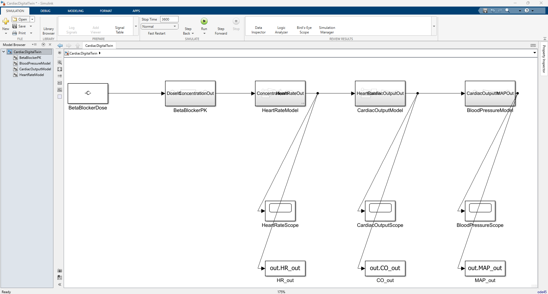
Block ID	Block	Interface
blk_1	BetaBlockerDose (Constant)	out: scalar dose value in mg
blk_2	BetaBlockerPK	in: DoseIn (mg). out: ConcentrationOut (plasma drug level)
blk_3	HeartRateModel	in: ConcentrationIn, BaroreflexIn (bpm correction). out: HeartRateOut (bpm)
blk_4	CardiacOutputModel	in: HeartRateIn. out: CardiacOutputOut (L/min)
blk_5	BloodPressureModel	in: CardiacOutputIn. out: MAPOut (mmHg)
blk_6	BaroreflexController	in: MAPIn (mmHg). out: HRCorrectionOut (bpm)

What blk_N means

Every block in Simulink has a stable internal ID like blk_2. The MCP tools Copilot uses (model_read, model_edit, model_query_params) refer to blocks by these IDs, which is why they show up in the documentation. You can ignore them if you only care about the named blocks.

---

Subsystem details

BetaBlockerPK: first-order pharmacokinetics

flowchart LR
    DoseIn -->|D| TF["Transfer Fcn<br/>1 / (τ·s + 1)"] -->|C| ConcentrationOut

This subsystem models pharmacokinetics (PK): how the concentration of a drug in the blood changes over time after you take it. The single block inside is a continuous-time transfer function, the Simulink way to write a linear differential equation:

PKTransferFcn:
  Numerator   = [1]
  Denominator = [pk_time_constant 1]   % = [1800  1]

In plain words, after you take the metoprolol tablet, the level of the drug in your blood (the plasma concentration) rises smoothly toward a plateau equal to the dose. It does not jump there instantly. It approaches the plateau on an exponential curve.

A few engineering details that matter for the demo.

The DC gain (the ratio between input and output once everything has settled) is one. At steady state the plasma concentration equals the dose value. This is what lets the validation test drive the HeartRateModel subsystem directly with const(50) and const(60) on ConcentrationIn (holding BaroreflexIn at const(0) to isolate the open-loop drug effect) and still represent the forward-path comparison.

The time constant \(\tau = 1800\) s, equivalent to 30 minutes. The time constant tells you how fast the system responds. After one \(\tau\), the response has reached about 63 % of its final value. After 5\(\tau\) (9000 s, 2.5 hours), it is within 0.7 % of the final value. The simulation's default StopTime of 3600 s catches roughly 86 % of the asymptote (2 time constants); the full-validation runs extend to 9000 s.

The half-life is \(\tau \ln 2\), about 21 minutes. Metoprolol's clinical half-life is actually 3 to 7 hours. The demo uses 30 minutes so the simulation does not take all day, while preserving the exponential shape of the response.

HeartRateModel: chronotropic response

flowchart LR
    ConcentrationIn --> Hill["Fcn: HillEquation<br/>Emax·Cⁿ / (EC50ⁿ + Cⁿ)<br/>(18, 35, 1.5)"]
    Baseline["Constant<br/>baseline_heart_rate (75 bpm)"]
    BaroreflexIn["BaroreflexIn<br/>(HR correction, bpm)"]
    Hill --> Sum["Σ<br/>− drug + baro"]
    Baseline --> Sum
    BaroreflexIn --> Sum
    Sum --> Sat["Saturation<br/>[40, 180] bpm"]
    Sat --> HeartRateOut

The subsystem combines a baseline rate, a nonlinear drug effect, and the baroreflex correction, then clamps the result: Constant, Fcn (the Hill curve), Sum, Saturation, plus the two Inports and one Outport that connect it to its neighbours.

\[ \text{HR}(t) = \mathrm{clamp}\!\left(\text{HR}_0 - E_{\max}\frac{C(t)^n}{EC_{50}^n + C(t)^n} + \Delta\text{HR}_\text{baro}(t),\ 40,\ 180\right) \]

The clinical term chronotropic means "affecting heart rate". Beta-blockers reduce heart rate by occupying beta-1 receptors on the cardiac pacemaker cells that would otherwise be stimulated by adrenaline. That binding saturates: once most receptors are occupied, additional drug adds little further effect. The HillEquation Fcn block captures this with the standard Hill/Emax curve (\(E_{\max} = 18\) bpm ceiling, \(EC_{50} = 35\) mg half-maximal concentration, Hill coefficient \(n = 1.5\)). See Advanced physiology for the full treatment.

The second input, BaroreflexIn, carries the heart-rate correction from the BaroreflexController subsystem, closing the autonomic feedback loop. When MAP falls, the baroreflex adds a positive HR correction that partially restores rate.

The Saturation block sets a physiological floor and ceiling on the heart rate. It is a defensive guard, not an active part of normal operation: at the standard doses the clamp never engages.

CardiacOutputModel: a Fick-like product

flowchart LR
    HeartRateIn -->|HR| Prod["×"]
    SV["Constant<br/>stroke_volume_mL (70)"] --> Prod
    Prod --> Conv["× 1/1000<br/>(mL → L)"]
    Conv --> CardiacOutputOut

\[ \text{CO}\ [\text{L/min}] = \text{HR}\ [\text{bpm}] \times \frac{\text{SV}\ [\text{mL}]}{1000} \]

Cardiac output (CO) is the total volume of blood the heart pumps per minute. It is a direct multiplication: how many heartbeats per minute, times how much blood per heartbeat. The × 1/1000 is a unit conversion from millilitres to litres.

Stroke volume (SV) is the amount of blood ejected with each beat (about 70 mL at rest for a typical adult). Beta-blockers' impact on stroke volume is small and goes in two directions at once: a slower heart has more time to fill (which slightly increases SV) but also contracts a little less forcefully (which slightly decreases SV). For a first-order picture, treating SV as a fixed parameter is honest. A more complex model would tie SV to the Frank-Starling relationship, where SV depends on how much blood enters the heart before each beat.

BloodPressureModel: afterload coupling

flowchart LR
    CardiacOutputIn -->|CO| Gain["× svr_mmHg_min_per_L<br/>(18)"]
    Gain --> MAPOut

\[ \text{MAP}\ [\text{mmHg}] = \text{CO}\ [\text{L/min}] \cdot \text{SVR}\ [\text{mmHg}\cdot\text{min/L}] \]

A direct application of the haemodynamic identity that ties mean blood pressure to flow and resistance. MAP (mean arterial pressure) is the time-averaged pressure in the arteries. SVR (systemic vascular resistance) is how much the body's blood vessels resist that flow, sometimes called the afterload because it is the load the heart has to pump against.

SVR is held constant in this model. Beta-blockers have very little direct effect on blood vessels at this dose; the pressure drop they produce comes almost entirely from the cardiac output drop, not from vessel dilation.

---

Why this structure (and not something else)

The model balances physiological realism against legibility for a live demo. It includes the two effects that matter most for a dose-change question — saturating receptor binding and the baroreflex — while leaving out complexity that would not change the steady-state answer. The deeper treatment is in Advanced physiology.

Modelling choice	Rationale
Hill/Emax receptor-binding PD (dose-response saturates at high doses)	Included. Captures the diminishing returns that make the 50→60 mg marginal effect small and clinically realistic.
Closed-loop baroreflex (the body's automatic blood-pressure feedback that nudges HR when MAP changes)	Included. Adds the autonomic feedback that keeps MAP from falling unrealistically far and attenuates the dose-to-HR gain.
Two-compartment PK (drug distributes into a peripheral tissue compartment as well as the blood)	Omitted. Captures distribution kinetics that are not needed for a steady-state dose-change question. The one-compartment model gives the same steady state and the right transient shape.
Stateflow control logic	Omitted. Belongs in a closed-loop controller demo, not a plant model.

Every parameter has units, a clinical reference, and a clear role in one formula. That traceability is what makes the Copilot workflow legible for the live demo, even with the nonlinearity and feedback in place.

---

How the model is built

The .slx file is gitignored. Whoever clones this repo regenerates it from the source script:

run('model/create_cardiac_model.m')

That script does the following.

1. Loads the workspace parameters by running model/cardiac_params.m.
2. Creates a fresh CardiacDigitalTwin system.
3. Configures the solver (ode45, variable-step, StopTime = 3600). The solver is the numerical algorithm that integrates the model equations forward in time; variable-step means it picks its own time step to maintain accuracy.
4. Adds the dose Constant block bound to beta_blocker_dose_mg (a workspace variable, so it can be changed from MATLAB without editing the model).
5. Adds each subsystem with named Inport and Outport blocks, including the BaroreflexController and the second BaroreflexIn inport on HeartRateModel.
6. Wires the internals of every subsystem and closes the baroreflex loop from BloodPressureModel back into HeartRateModel.
7. Adds Scope and To Workspace blocks at the root.
8. Saves the resulting CardiacDigitalTwin.slx.

The source of truth for a Simulink model is far more reviewable when it is a script than when it is a binary .slx. Diffs become readable. Merges become tractable. The model's structure is documented by being the script that builds it. This is also the pattern that makes Copilot most useful: when the model is buildable from text, Copilot can reason about, edit, and regenerate it without ever needing to manipulate the binary directly.

---

Top-level outputs

The three Scopes are for live viewing during simulation. The three To Workspace blocks are for analysis after the run completes. They are stored in SaveFormat = 'Array', which gives a plain column vector of values. Time is recovered from the tout companion variable that Simulink automatically populates.

Variable	Source block	Shape after a 9000 s run
tout	tout (model logging)	N × 1 (the variable-step solver decides N)
HR_out	HeartRateModel → HR_out	N × 1 bpm
CO_out	CardiacOutputModel → CO_out	N × 1 L/min
MAP_out	BloodPressureModel → MAP_out	N × 1 mmHg

This is the format the real-time dashboard reads and the validation tests inspect. The same plumbing supports both interactive exploration and automated verification.